Design

• 1: Ciphertext Management
• 2: Ciphertext Packing System
• 3: Data-oblivious Transformations
• 4: Noise Analysis
• 5: Secret
• 6: SIMD Optimizations
• 7: Optimizing relinearization

HEIR is a compiler toolchain that allows the compilation of high-level programs to equivalent programs that operate on encrypted data.

HEIR is built in the MLIR framework.

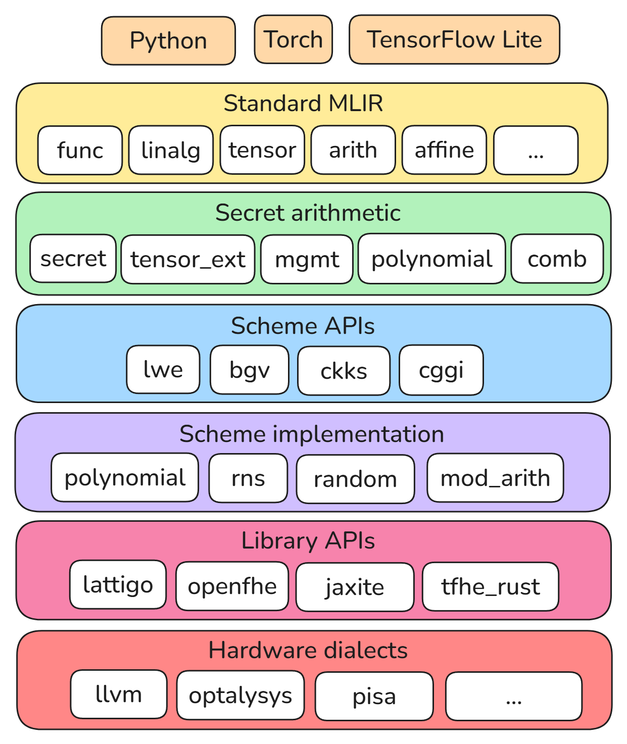
HEIR defines dialects at various layers of abstraction, from high-level scheme-agnostic operations on secret types to low-level polynomial arithmetic. The diagram below shows some of the core HEIR dialects, and the compilation flow is generally from the top of the diagram downward.

The pages in this section describe the design of various subcomponents of HEIR.

1 - Ciphertext Management

On 2025-04-17, Hongren Zheng gave a talk overview of the ciphertext management system in the HEIR working group meeting. The video can be found here and the slides can be found here

Introduction

To lower from user specified computation to FHE scheme operations, a compiler must insert ciphertext management operations to satisfy various requirements of the FHE scheme, like modulus switching, relinearization, and bootstrapping. In HEIR, such operations are modeled in a scheme-agnostic way in the mgmt dialect.

Taking the arithmetic pipeline as example: a program specified in high-level MLIR dialects like arith and linalg is first transformed to an IR with only arith.addi/addf, arith.muli/mulf, and tensor_ext.rotate operations. We call this form the secret arithmetic IR.

Then management passes insert mgmt ops to support future lowerings to scheme dialects like bgv and ckks. As different schemes have different management requirement, they should be inserted in different styles.

We discuss each scheme below to show the design in HEIR. For RLWE schemes, we all assume RNS instantiation.

BGV

BGV is a leveled scheme where each level has a modulus $q_i$. The level is numbered from $0$ to $L$ where $L$ is the input level and $0$ is the output level. The core feature of BGV is that when the magnititude of the noise becomes large (often caused by multiplication), a modulus switching operation from level $i$ to level $i-1$ can be inserted to reduce the noise to a “constant” level. In this way, BGV can support a circuit of multiplicative depth $L$.

BGV: Relinearization

HEIR initially inserts relinearization ops immediately after each multiplication to keep ciphertext dimension “linear”. A later relinearization optimization pass relaxes this requirement, and uses an integer linear program to decide when to relinearize. See Optimizing Relinearization for more details.

BGV: Modulus switching

There are several techniques to insert modulus switching ops.

For the example circuit input -> mult -> mult -> output, the insertion result could be one of

1. After multiplication: input -> (mult -> ms) -> (mult -> ms) -> output

2. Before multiplication: input -> (mult) -> (ms -> mult) -> (ms -> output)

3. Before multiplication (including the first multiplication): input -> (ms -> mult) -> (ms -> mult) -> (ms -> output)

The first strategy is from the BGV paper, the second and third strategies are from OpenFHE, which correspond to the FLEXIBLEAUTO mode and FLEXIBLEAUTOEXT mode, respectively.

The first strategy is conceptually simpler, yet other policies have the advantage of smaller noise growth. In latter policies, by delaying the modulus switch until just before multiplication, the noise from other operations between multiplications (like rotation/relinearization) also benefit from the noise reduction of a modulus switch.

Note that, as multiplication has two operands, the actual circuit for the latter two policies is mult(ms(ct0), ms(ct1)), whereas in the first policy the circuit is ms(mult(ct0, ct1)).

The third policy has one more switching op than the others, so it will need one more modulus.

There are also other insertion strategy like inserting it dynamically based on current noise (see HElib) or lazy modulus switching. Those are not implemented.

BGV: Scale management

For the original BGV scheme, it is required to have $qi \equiv 1 \pmod{t}$ where $t$ is the plaintext modulus. However in practice such requirement will make the choice of $q_i$ too constrained. In the GHS variant, this condition is removed, with the price of scale management needed.

Modulus switching from level $i$ to level $i-1$ is essentially dividing (with rounding) the ciphertext by $q_i$, hence dividing the noise and payload message inside by $q_i$. The message $m$ can often be written as $[m]_t$, the coset representative of m $\mathbb{Z}/t\mathbb{Z}$. Then by dividing of $q_i$ produces a result message $[m \cdot q_i^{-1}]_t$.

Note that when $qi \equiv 1 \pmod{t}$, the result message is the same as the original message. However, in the GHS variant this does not always hold, so we call the introduced factor of $[q^{-1}]_t$ the scale of the message. HEIR needs to record and manage it during compilation. When decrypting the scale must be removed to obtain the right message.

Note that, for messages $m_0$ and $m_1$ of different scale $a$ and $b$, we cannot add them directly because $[a \cdot m_0 + b \cdot m_1]_t$ does not always equal $[m_0 + m_1]_t$. Instead we need to adjust the scale of one message to match the other, so $[b \cdot m_0 + b \cdot m_1]_t = [b \cdot (m_0 + m_1)]_t$. Such adjustment could be done by multiplying $m_0$ with a constant $[b \cdot a^{-1}]_t$. This adjustment is not for free, and increases the ciphertext noise.

As one may expect, different modulus switching insertion strategies affect message scale differently. For $m_0$ with scale $a$ and $m_1$ with scale $b$, the result scale would be

1. After multiplication: $[ab / qi]_t$.

2. Before multiplication: $[a / qi \cdot b / qi]_t = [ab / (qi^2)]_t$.

This is messy enough. To ease the burden, we can impose additional requirement: mandate a constant scale $\Delta_i$ for all ciphertext at level $i$. This is called the level-specific scaling factor. With this in mind, addition within one level can happen without caring about the scale.

1. After multiplication: $\Delta_{i-1} = [\Delta_i^2 / qi]_t$

2. Before multiplication: $\Delta_{i-1} = [\Delta_i^2 / (qi^2)]_t$

BGV: Cross Level Operation

With the level-specific scaling factor, one may wonder how to perform addition and multiplication of ciphertexts on different levels. This can be done by adjusting the level and scale of the ciphertext at the higher level.

The level can be easily adjusted by dropping the extra limbs, and scale can be adjusted by multiplying a constant, but because multiplying a constant will incur additional noise, the procedure becomes the following:

1. Assume the level and scale of two ciphertexts are $l_1$ and $l_2$, $s_1$ and $s_2$ respectively. WLOG assume $l_1 > l_2$.

2. Drop $l_1 - l_2 - 1$ limbs for the first ciphertext to make it at level $l_2 + 1$, if those extra limbs exist.

3. Adjust scale from $s_1$ to $s_2 \cdot q_{l_2 + 1}$ by multiplying $[s_2 \cdot q_{l_2 + 1} / s1]_t$ for the first ciphertext.

4. Modulus switch from $l_2 + 1$ to $l_2$, producing scale $s_2$ for the first ciphertext and its noise is controlled.

BGV: Implementation in HEIR

In HEIR the different modulus switching policy is controlled by the pass option for --secret-insert-mgmt-bgv. The pass defaults to the “Before Multiplication” policy. If user wants other policy, the after-mul or before-mul-include-first-mul option may be used. The mlir-to-bgv pipeline option modulus-switch-before-first-mul corresponds to the latter option.

The secret-insert-mgmt pass is also responsible for managing cross-level operations. However, as the scheme parameters are not generated at this point, the concrete scale could not be instantiated so some placeholder operations are inserted.

After the modulus switching policy is applied, the generate-param-bgv pass generates scheme parameters. Optionally, user could skip this pass by manually providing scheme parameter as an attribute at module level.

Then populate-scale-bgv comes into play by using the scheme parameters to instantiate concrete scale, and turn those placeholder operations into concrete multiplication operation.

CKKS

CKKS is a leveled scheme where each level has a modulus $q_i$. The level is numbered from $0$ to $L$ where $L$ is the input level and $0$ is the output level. CKKS ciphertext contains a scaled message $\Delta m$ where $\Delta$ takes some value like $2^40$ or $2^80$. After multiplication of two messages, the scaling factor $\Delta’$ will become larger, hence some kind of management policy is needed in case it blows up. Contrary to BGV where modulus switching is used for noise management, in CKKS modulus switching from level $i$ to level $i-1$ can divide the scaling factor $\Delta$ by the modulus $q_i$.

The management of CKKS is similar to BGV above in the sense that their strategy are the similar and uses similar code base. However, BGV scale management is internal and users are not required to concern about it, while CKKS scale management is visible to user as it affects the precision. One notable difference is that, for “Before multiplication (including the first multiplication)” modulus switching policy, the user input should be encoded at $\Delta^2$ or higher, as otherwise the first modulus switching (or rescaling in CKKS term) will rescale $\Delta$ to $1$, rendering full precision loss.

2 - Ciphertext Packing System

This document describes HEIR’s ciphertext packing system, including:

• A notation and internal representation of a ciphertext packing, which we call a layout.
• An abstraction layer to associate SSA values with layouts and manipulate and analyze them before a program is converted to concrete FHE operations.
• A variety of layouts and kernels from the FHE literature.
• A layout and kernel optimizer based on the Fhelipe compiler.
• A layout conversion implementation of the Vos-Vos-Erkin graph coloring algorithm.

For background on what ciphertext packing is and its role in homomorphic encryption, see this introductory blog post. The short version of that blog post is that the SIMD-style HE computational model requires implementing linear-algebraic operations in terms of elementwise additions, multiplications, and cyclic rotations of large-dimensional vectors (with some exceptions like the Park-Gentry matrix-multiplication kernel).

Practical programs require many such operations, and the task of the compiler is to jointly choose ciphertext packings and operation kernels so as to minimize overall program latency. In this document we will call the joint process of optimizing layouts and kernels by the name “layout optimization.” In FHE programs, runtime primarily comes from the quantity of rotation and bootstrap operations, the latter of which is in turn approximated by multiplicative depth. Metrics like memory requirements may also be constrained, but for most of this document latency is the primary concern.

HEIR’s design goal is to be an extensible HE compiler framework, we aim to support a variety of layout optimizers and multiple layout representations. As such, we separate the design of the layout representation from the details of the layout optimizer, and implement lowerings for certain ops that can be reused across optimizers.

This document will begin by describing the layout representation, move on to the common, reusable components for working with that representation, and then finally describe one layout optimizer implemented in HEIR based on Fhelipe.

Layout representation

A layout is a description of how cleartext data is organized within a list of ciphertexts. In general, a layout is a partial function mapping from the index set of a list of ciphertext slots to the index set of a cleartext tensor. The function describes which cleartext data value is stored at which ciphertext slot.

A layout is partial because not all ciphertext slots need to be used, and the function uses ciphertext slots as the domain and cleartext indices as the codomain because cleartext values may be replicated among multiple slots, but a slot can store at most one cleartext value.

HEIR restricts the above definition of a layout as follows:

• The partial function must be expressible as a Presburger relation, which will be defined in detail below.
• Unmapped ciphertext slots always contain zero.

We claim that this subset of possible layouts is a superset of all layouts that have been used in the FHE literature to date. For example, both the layout notation of Fhelipe and the TileTensors of HeLayers are defined in terms of specific parameterized quasi-affine formulas.

Next we define a Presburger relation, then move on to examples.

Quasi-affine formulas and Presburger relations

Definition: A quasi-affine formula is a multivariate formula built from the following operations:

• Integer literals
• Integer-valued variables
• addition and subtraction
• multiplication by an integer constant
• floor- and ceiling-rounded division by a nonzero integer constant
• modulus by a nonzero integer constant

Using the BNF grammar from the MLIR website, we can also define it as

affine-expr ::= `(` affine-expr `)`
              | affine-expr `+` affine-expr
              | affine-expr `-` affine-expr
              | `-`? integer-literal `*` affine-expr
              | affine-expr `ceildiv` integer-literal
              | affine-expr `floordiv` integer-literal
              | affine-expr `mod` integer-literal
              | `-`affine-expr
              | bare-id
              | `-`? integer-literal

Definition: Let $d, r \in \mathbb{Z}_{\geq 0}$ represent a number of domain and range dimensions, respectively. A Presburger relation is a binary relation over $\mathbb{Z}^{d} \times \mathbb{Z}^{r}$ that can be expressed as the solution to a set of equality and inequality constraints defined using quasi-affine formulas.

We will use the Integer Set Library (ISL) notation to describe Presburger relations. For an introduction to the ISL notation and library, see this article. For a comprehensive reference, see the ISL manual.

Example 1: Given a data vector of type tensor<8xi32> and a ciphertext with 32 slots, a layout that repeats the tensor cyclically is given as:

{
    [d] -> [ct, slot] :
    0 <= d < 8
    and ct = 0
    and 0 <= slot < 32
    and (d - slot) mod 8 = 0
}

From Example 1, we note that in HEIR the domain of a layout always aligns with the shape of the domain tensor, and the range of a layout is always a 2D tensor whose first dimension denotes the ciphertext index and whose second index is the slot within that ciphertext.

Example 2: Given a data matrix of type tensor<8x8xi32> and 8 ciphertexts with 32 slots each, the following layout implements the standard Halevi-Shoup diagonal layout.

{
    [row, col] -> [ct, slot] :
    0 <= row < 8
    and 0 <= col < 8
    and 0 <= ct < 8
    and 0 <= slot < 32
    and (row - col + ct) mod 8 = 0
    and (row - slot) mod 32 = 0
}

Note, this layout implements a diagonal packing, and further replicates each diagonal cyclically within a ciphertext.

Layout attributes

Layouts are represented in HEIR via the tensor_ext.layout attribute. Its argument includes a string using the ISL notation above. For example

#tensor_layout = #tensor_ext.layout<
    "{ [i0] -> [ct, slot] : (slot - i0) mod 8 = 0 and ct = 0 and 1023 >= slot >= 0 and 7 >= i0 >= 0 }"
>

Generally, layout attributes are associated with an SSA value by being attached to the op that owns the SSA value. In MLIR, which op owns the value has two cases:

• For an op result, the layout attribute is stored on the op.
• For a block argument, the layout attribute is stored on the op owning the block, using the OperandAndResultAttrInterface to give a consistent API for accessing the attribute.

These two differences are handled properly by a helper library, lib/Utils/AttributeUtils.h, which exposes setters and getters for layout attributes. As of 2025-10-01, the system does not provide a way to handle ops with multiple regions or multi-block regions.

For example, #layout_attr is associated with the SSA value %1:

%1 = arith.addi %0, %1 {tensor_ext.layout = #layout_attr} : tensor<512xf32>

Data-semantic and ciphertext-semantic tensors

In HEIR, before lowering to scheme ops, we distinguish between types in two regimes:

• Data-semantic tensors, which are scalars and tensors that represent cleartext data values, largely unchanged from the original input program.
• Ciphertext-semantic tensors, which are rank-2 tensors that represent packed cleartext values in ciphertexts.

The task of analyzing an IR to determine which layouts and kernels to use happens in the data-semantic regime. In these passes, chosen layouts are persisted between passes as attributes on ops (see Layout attributes above), and data types are unchanged.

In this regime, there are three special tensor_ext ops that are no-ops on data-semantic type, but are designed to manipulate the layout attributes. These ops are:

• tensor_ext.assign_layout, which takes a data-semantic value and a layout attribute, and produces the same data-semantic type. This is an “entry point” into the layout system and lowers to a loop that packs the data according to the layout.
• tensor_ext.convert_layout, which makes an explicit conversion between a data-semantic value’s current layout and a new layout. Typically this lowers to a shift network.
• tensor_ext.unpack, which clears the layout attribute on a data-semantic value, and serves as an exit point from the layout system. This lowers to a loop which extracts the packed cleartext data back into user data.

A layout optimizer is expected to insert assign_layout ops for any server-side cleartexts that need to be packed at runtime.

In the ciphertext-semantic regime, all secret values are rank-2 tensors whose first axis indexes ciphertexts and whose second axis indexes slots within ciphertexts. These tensors are subject to the constraints of the SIMD FHE computational model (elementwise adds, muls, and structured rotations), though the type system does not enforce this until secret-to-<scheme> lowerings, which would fail if encountering an op that cannot be implemented in FHE.

We preserve the use of the tensor type here, rather than create new types, so that we can reuse MLIR infrastructure. For example, if we were to use a new tensor-like type for ciphertext-semantic tensors, we would not be able to use arith.addi anymore, and would have to reimplement folding and canonicalization patterns from MLIR in HEIR. In the future we hope MLIR will relax these constraints via interfaces and traits, and at that point we could consider a specialized type.

Before going on, we note that the layout specification language is agnostic to how the “slots” are encoded in the underlying FHE scheme. In particular, slots could correspond to evaluation points of an RNS polynomial, i.e., to “NTT form” slots. But they could also correspond to the coefficients of an RNS polynomial in coefficient form. As of 2025-10-01, HEIR’s Fhelipe-inspired pipeline materializes slots as NTT-form slots in all cases, but is not required by the layout system. The only part of the layout system that depends on NTT-form is the implementation of operation kernels in terms of rotation operations, as coefficient-form ciphertexts do not have a rotation operation available. Future layout optimizers may take into account conversions between NTT and coefficient form as part of a layout conversion step.

HEIR’s Fhelipe-inspired layout optimizer

Pipeline overview

The mlir-to-<scheme> pipeline involves the following passes that manipulate layouts:

• layout-propagation
• layout-optimization
• convert-to-ciphertext-semantics
• implement-rotate-and-reduce
• add-client-interface

The two passes that are closest to Fhelipe’s design are layout-propagation and layout-optimization. The former sets up initial default layouts for all values and default kernels for all ops that need them, and propagates them forward, inserting layout conversion ops as needed to resolve layout mismatches. The latter does a backwards pass, jointly choosing more optimal kernels and attempting to hoist layout conversions earlier in the IR. If layout conversions are hoisted all the way to function arguments then they are “free” because they can be merged into client preprocessing.

Next we will outline the responsibility of each pass in detail. The documentation page for each of these passes is linked in each section, and contains doctests as examples that are kept in sync with the implementation of the pass.

layout-propagation

The layout-propagation pass runs a forward pass through the IR to assign default layouts to each SSA value that needs one, and a default kernel to each operation that needs one.

For each secret-typed function argument, no layout can be inferred, so a default layout is assigned. The default layout for scalars is to repeat the scalar in every slot of a single ciphertext. The default layout for tensors is a row-major layout into as many ciphertexts as are needed to fit the tensor.

Then layouts are propagated forward through the IR. For each op, a default kernel is chosen, and if the layouts of the operands are already set and agree, the result layout is inferred according to the kernel.

If the layouts are not compatible with the default kernel, a convert_layout op is inserted to force compatibility. If one or more operands has a layout that is not set (which can happen if the operand is a cleartext value known to the server), then a compatible layout is chosen and an assign_layout op is inserted to persist this information for later passes.

Because layout-propagation may have inserted some redundant conversions, sequences of assign_layout followed by convert_layout are folded together into combined assign_layout ops.

layout-optimization

The layout-optimization pass has two main goals: to choose better kernels for ops, and to try to eliminate convert_layout ops. It does this by running a backward pass through the IR. If it encounters an op that is followed by a convert_layout op, it attempts to hoist the convert_layout through the op to its arguments.

In doing this, it must consider:

• Changing the kernel of the op, and the cost of implementing the kernel. E.g., a new kernel may be better for the new layout of the operands.
• Whether the new layout of op results still need to be converted, and the new cost of these conversions. E.g., if the op result has multiple uses, or the op result had multiple layout conversions, only one of which is hoisted.
• The new cost of operand layout conversions. E.g., if a layout conversion is hoisted to one operand, it may require other operands to be converted to remain compatible.

In all of the above, the “cost” includes an estimate of the latency of a kernel, an estimate of the latency of a layout conversion, as well as the knowledge that some layout conversions may be free or cheaper because of their context in the IR.

NOTE: The cost of a kernel is calculated using symbolic execution of kernel DAGs. The implementation uses a rotation-counting visitor that traverses the kernel’s arithmetic DAG with CSE deduplication (see lib/Kernel/RotationCountVisitor.h). The cost accounts for rotation operations, which dominate FHE latency. Currently, only rotation costs are modeled; multiplication depth is not yet included.

The cost of a layout conversion is estimated by simulating what the implement-shift-network would do if it ran on a layout conversion. And layout-optimization includes analyses that allow it to determine a folded cost for layout conversions that occur after other layout conversions, as well as the free cost of layout conversions that occur at function arguments, after assign_layout ops, or separated from these by ops that do not modify a layout.

After the backward pass, any remaining convert_layout ops at the top of a function are hoisted into function arguments and folded into existing layout attributes.

convert-to-ciphertext-semantics

The convert-to-ciphertext-semantics pass has two responsibilities that must happen at the same time:

• Converting all data-semantic values to ciphertext-semantic values with corresponding types.
• Implementing FHE kernels for all ops as chosen by earlier passes.

After this pass is complete, the IR must be in the ciphertext-semantic regime and all operations on secret-typed values must be constrained by the SIMD FHE computational model.

In particular, this pass implements assign_layout as an explicit loop that packs cleartext data into ciphertext slots according to the layout attribute. It also implements convert_layout as a shift network, which is a sequence of plaintext masks and rotations that can arbitrarily (albeit expensively) shuffle data in slots. This step can be isolated via the implement-shift-network pass, but the functionality is inlined in this pass since it must happen at the same time as type conversion.

When converting function arguments, any secret-typed argument is assigned a new attribute called tensor_ext.original_type, which records the original data-semantic type of the argument as well as the layout used for its packing. This is used later by the add-client-interface pass to generate client-side encryption and decryption helper functions.

implement-rotate-and-reduce

Some kernels rely on a baby-step giant-step optimization, and defer the implementation of that operation so that canonicalization patterns can optimize them. Instead they emit a tensor_ext.rotate_and_reduce op. The implement-rotate-and-reduce pass implements this op using baby-step giant-step, or other approaches that are relevant to special cases.

add-client-interface

The add-client-interface pass inserts additional functions that can be used by the client to encrypt and decrypt data according to the layouts chosen by the layout optimizer.

It fetches the original_type attribute on function arguments, and generates an encryption helper function for each secret argument, and a decryption helper function for each secret return type.

These helper functions use secret.conceal and secret.reveal for scheme-agnostic encryption and decryption, but eagerly implement the packing logic as a loop, equivalently to how assign_layout is lowered in convert-to-ciphertext-semantics, and adding an analogous lowering for tensor_ext.unpack.

Reusable components for working with layouts

Lowering data-semantic ops with FHE kernels

Any layout optimizer will eventually need to convert data-semantic values to ciphertext-semantic tensors. In doing this, all kernels need to be implemented in one pass at the same time that the types are converted.

The convert-to-ciphertext-semantics pass implements this conversion without making any decisions about which layouts or kernels to use. In particular, for ops that have multiple supported kernels, it picks the kernel to use based on the kernel attribute on the op (cf. secret::SecretDialect::kKernelAttrName).

In this way, we decouple the decision of which layout and kernel to use (the optimizer’s job) from the implementation of that kernel (the lowering’s job). Ideally all layout optimizer pipelines can reuse this pass, which avoids the common pitfalls associated with writing dialect conversion passes. New kernels, similarly, can be primarily implemented as described in the next section.

Finally, if a new optimizer or layout notation is introduced into HEIR, it should ultimately be converted to use the same tensor_ext.layout attribute so that it can reuse the lowerings of ops like tensor_ext.assign_layout and tensor_ext.unpack.

Testing kernels and layouts

Writing kernels can be tricky, so HEIR provides a simplified framework for implementing kernels which allows them to be unit-tested in isolation, while the lowering to MLIR is handled automatically by a common library.

The implementation library is called ArithmeticDag. Some initial implementations are in lib/Kernel/KernelImplementation.h, and example unit tests are in lib/Kernel/*Test.cpp. Then a class called IRMaterializingVisitor walks the DAG and generates MLIR code.

Similarly, lib/Utils/Layout/Evaluate.h provides helper functions to materialize layouts on test data-semantic tensors, which can be combined with ArithmeticDag to unit-test a layout and kernel combination without ever touching MLIR.

Manipulating layouts

The directory lib/Utils/Layout contains a variety of helper code for manipulating layout relations, including:

• Constructing or testing for common kinds of layouts, such as row-major, diagonal, and layouts related to particular machine learning ops like convolution.
• Generating explicit loops that iterate over the space of points in a layout, which is used to generate packing and unpacking code.
• Helpers for hoisting layout conversions through ops.

These are implemented using two APIs: one is the Fast Presburger Library (FPL), which is part of MLIR and includes useful operations like composing relations and projecting out dimensions. The other is the Integer Set Library (ISL), which is a more fully-featured library that supports code generation and advanced analyses and simplification routines. As we represent layouts as ISL strings, we include a two-way interoperability layer that converts between ISL and FPL representations of the same Presburger relation.

A case study: the Orion convolution kernel

The Orion compiler presents a kernel for 2D convolution that first converts the filter input into a Toeplitz matrix $A$, and then applies a Halevi-Shoup diagonal packing and kernel on $A$ using the encrypted image vector $v$ packed row-major into a single ciphertext.

We describe how this layout is constructed and represented in HEIR.

The first, analytical step, is to describe a Presburger relation mapping a cleartext filter matrix to the Toeplitz matrix form as described in the Orion paper. Essentially, this involves writing down the loop nest that implements a convolution and, for each visited index,

Let $P$ be an integer padding value, fix stride 1, and define $i_{dr}, i_{dc}$ to be indices over the “data row” and “data column”, respectively, i.e., these variables track the top-left index of the filter as it slides over the convolved image in the data-semantic domain. For an image of height $H_d$ and width $W_d$, and a filter of height $H_f$ and width $W_f$, we have

$$ -P \leq i_{dr} \leq H_d + P - W_f $$

and similarly for $i_{dc}$.

Then we have bounds for the iteration of entries of the filter itself, for a fixed position of the filter over the image. If we consider these local variables $i_{fr}$ and $i_{fc}$ for “filter row” and “filter column”, respectively, we have

$$ 0 \leq i_{fr} < H_f $$

and similarly for $i_{fc}$.

From these two indices we can compute the corresponding entry of the data matrix that is being operated on as $i_{dr} + i_{fr}$ and $i_{dc} + i_{fc}$. If that index is within the bounds of the image, then the filter entry at that position is included in the Toeplitz matrix.

Finally, we need to compute the row and column of the Toeplitz matrix that each filter entry maps to. This is the novel part of the Orion construction. Each row of the Toeplitz matrix corresponds to one iteration over the filter (the filter is fixed at some position of the filter over the image). And the column value is a flattened index of the filter entry, plus offsets from both the padding and the iteration of the filter over the image (each step the filter moves adds one more to the offset).

The formula for the target row is

$$ m_{r} = (i_{dr} + P) F + i_{dc} + P $$

where $F$ is the total number of positions the filter assumes within each row, i.e., $F = H_d + 2P - H_f + 1$.

And the target column is

$$ m_{c} = W_d i_{dr} + i_{dc} + W_d i_{fr} + i_{fc} $$

Note the use of W_d for both the offset from the filter’s position over the image, and the offset from the filter’s own row.

Together this produces the following almost-Presburger relation:

[Hd, Wd, Hf, Wf, P] -> {
    [ifr, ifc] -> [mr, mc] : exists idr, idc :

    // Bound the top-left index of the filter as it slides over the image
    -P <= idr <= Hd + P - Hf
    and -P <= idc <= Wd + P - Wf

    // Bound the index within the filter
    and 0 <= ifr < Hf
    and 0 <= ifc < Wf

    // Only map values when the filter index is in bounds
    and 0 <= ifr + idr < Hd
    and 0 <= ifc + idc < Wd

    // Map the materialized filter index to its position in the Toeplitz matrix
    and mr = (idr + P) * (Wd + 2P - Wf + 1) + idc + P
    and mc = (idr * Wd + idc) + Wd * ifr + ifc
}

This is “almost” a Presburger relation because, even though the symbol variables Hd, Wd, Hf, Wf, and P are all integer constants, they cannot be multiplied together in a Presburger formula. But if we replace them with specific constants, such as

Hd = 8
Wd = 8
Hf = 3
Wf = 3
P = 1

We get

{
    [ifr, ifc] -> [mr, mc] : exists idr, idc :
    -1 <= idr <= 6
    and -1 <= idc <= 6
    and 0 <= ifr < 3
    and 0 <= ifc < 3
    and 0 <= ifr + idr < 8
    and 0 <= ifc + idc < 8
    and mr = (idr + 1) * 8 + idc + 1
    and mc = idr * 8 + idc + ifc + ifr * 8
}

Which ISL simplifies to

{
    [ifr, ifc] -> [mr, mc = -9 + 8ifr + ifc + mr] :
    0 <= ifr <= 2
    and 0 <= ifc <= 2
    and mr >= 0
    and 8 - 8ifr <= mr <= 71 - 8ifr
    and mr <= 63
    and 8*floor((mr)/8) >= -8 + ifc + mr
    and 8*floor((mr)/8) < ifc + mr
}

Next, we can compose the above relation with the Halevi-Shoup diagonal layout (using FPL’s IntegerRelation::compose), to get a complete layout from filter entries to ciphertext slots. Using ciphertexts with 1024 slots, we get:

{
    [ifr, ifc] -> [ct, slot] :
    (9 - 8ifr - ifc + ct) mod 64 = 0
    and 0 <= ifr <= 2
    and 0 <= ifc <= 2
    and 0 <= ct <= 63
    and 0 <= slot <= 1023
    and 8*floor((slot)/8) >= -8 + ifc + slot
    and 8*floor((slot)/8) < ifc + slot
    and 64*floor((slot)/64) >= -72 + 8ifr + ifc + slot
    and 64*floor((slot)/64) >= -71 + 8ifr + slot
    and 64*floor((slot)/64) <= -8 + 8ifr + slot
    and 64*floor((slot)/64) <= -9 + 8ifr + ifc + slot
}

FAQ

Can users define kernels without modifying the compiler?

No (as of 2025-10-01). However, a kernel DSL is in scope for HEIR. Reach out if you’d like to be involved in the design.

3 - Data-oblivious Transformations

A data-oblivious program is one that decouples data input from program execution. Such programs exhibit control-flow and memory access patterns that are independent of their input(s). This programming model, when applied to encrypted data, is necessary for expressing FHE programs. There are 3 major transformations applied to convert a conventional program into a data-oblivious program:

(1) If-Transformation

If-operations conditioned on inputs create data-dependent control-flow in programs. scf.if operations should at least define a ’then’ region (true path) and always terminate with scf.yield even when scf.if doesn’t produce a result. To convert a data-dependent scf.if operation to an equivalent set of data-oblivious operations in MLIR, we hoist all safely speculatable operations in the scf.if operation and convert the scf.yield operation to an arith.select operation. The following code snippet demonstrates an application of this transformation.

// Before applying If-transformation
func.func @my_function(%input : i1 {secret.secret}) -> () {
  ...
  // Violation: %input is used as a condition causing a data-dependent branch
  %result =`%input -> (i16) {
        %a = arith.muli %b, %c : i16
        scf.yield %a : i16
      } else {
        scf.yield %b : i16
      }
  ...
}

// After applying If-transformation
func.func @my_function(%input : i16 {secret.secret}) -> (){
  ...
  %a = arith.muli %b, %c : i16
  %result = arith.select %input, %a, %b : i16
  ...
}

We implement a ConvertIfToSelect pass that transforms operations with secret-input conditions and with only Pure operations (i.e., operations that have no memory side effect and are speculatable) in their body. This transformation cannot be applied to operations when side effects are present in only one of the two regions. Although possible, we currently do not support transformations for operations where both regions have operations with matching side effects. When side effects are present, the pass fails.

(2) Loop-Transformation

Loop statements with input-dependent conditions (bounds) and number of iterations introduce data-dependent branches that violate data-obliviousness. To convert such loops into a data-oblivious version, we replace input-dependent conditionals (bounds) with static input-independent parameters (e.g. defining a constant upper bound), and early-exits with update operations where the value returned from the loop is selectively updated using conditional predication. In MLIR, loops are expressed using either affine.for, scf.for or scf.while operations.

[!NOTE] Early exiting from loops is not supported in scf and affine, so early exits are not supported in this pipeline. Early exits are expected to be added to MLIR upstream at some point in the future.

• affine.for: This operation lends itself well to expressing data oblivious programs because it requires constant loop bounds, eliminating input-dependent limits.

 %sum_0 = arith.constant 0.0 : f32
 // The for-loop's bound is a fixed constant
 %sum = affine.for %i = 0 to 10 step 2
 iter_args(%sum_iter = %sum_0) -> (f32) {
   %t = affine.load %buffer[%i] : memref<1024xf32>
   %sum_next = arith.addf %sum_iter, %input : f32
   affine.yield %sum_next : f32
 }
 ...

• scf.for: In contrast to affine.for, scf.for does allow input-dependent conditionals which does not adhere to data-obliviousness constraints. A solution to this could be to either have the programmer or the compiler specify an input-independent upper bound so we can transform the loop to use this upper bound and also carefully update values returned from the for-loop using conditional predication. Our current solution to this is for the programmer to add the lower bound and worst case upper bound in the static affine loop’s attributes list.

func.func @my_function(%value: i32 {secret.secret}, %inputIndex: index {secret.secret}) -> i32 {
  ...
  // Violation: for-loop uses %inputIndex as upper bound which causes a secret-dependent control-flow
  %result = scf.for %iv = %begin to %inputIndex step %step_value iter_args(%arg1 = %value) -> i32 {
    %output = arith.muli %arg1, %arg1 : i32
    scf.yield %output : i32
  }{lower = 0, upper = 32}
  ...
}

// After applying Loop-Transformation
func.func @my_function(%value: i32 {secret.secret}, %inputIndex: index {secret.secret}) -> i32 {
  ...
  // Build for-loop using lower and upper values from the `attributes` list
  %result = affine.for %iv = 0 to  step 32 iter_args(%arg1 = %value) -> i32 {
    %output = arith.muli %arg1, %agr1 : i32
    %cond = arith.cmpi eq, %iv, %inputIndex : index
    %newOutput = arith.select %cond, %output, %arg1
    scf.yield %newOutput : i32
    }
  ...
}

• scf.while: This operation represents a generic while/do-while loop that keeps iterating as long as a condition is met. An input-dependent while condition introduces a data-dependent control flow that violates data-oblivious constraints. For this transformation, the programmer needs to add the max_iter attribute that describes the maximum number of iterations the loop runs which we then use the value to build our static affine.for loop.

// Before applying Loop-Transformation
func.func @my_function(%input: i16 {secret.secret}){
  %zero = arith.constant 0 : i16
  %result = scf.while (%arg1 = %input) : (i16) -> i16 {
    %cond = arith.cmpi slt, %arg1, %zero : i16
    // Violation: scf.while uses %cond whose value depends on %input
    scf.condition(%cond) %arg1 : i16
  } do {
  ^bb0(%arg2: i16):
    %mul = arith.muli %arg2, %arg2: i16
    scf.yield %mul
  } attributes {max_iter = 16 : i64}
  ...
  return
}

// After applying Loop-Transformation
func.func @my_function(%input: i16 {secret.secret}){
  %zero = arith.constant 0 : i16
  %begin = arith.constant 1 : index
  ...
  // Replace while-loop with a for-loop with a constant bound %MAX_ITER
  %result = affine.for %iv = %0 to %16 step %step_value iter_args(%iter_arg = %input) -> i16 {
    %cond = arith.cmpi slt, %iter_arg, %zero : i16
    %mul = arith.muli %iter_arg, %iter_arg : i16
    %output = arith.select %cond, %mul, %iter_arg
    scf.yield %output
  }{max_iter = 16 : i64}
  ...
  return
}

(3) Access-Transformation

Input-dependent memory access cause data-dependent memory footprints. A naive data-oblivious solution to this maybe doing read-write operations over the entire data structure while only performing the desired save/update operation for the index of interest. For simplicity, we only look at load/store operations for tensors as they are well supported structures in high-level MLIR likely emitted by most frontends. We drafted the following non-SIMD approach for this transformation and defer SIMD optimizations to the heir-simd-vectorizer pass:

// Before applying Access Transformation
func.func @my_function(%input: tensor<16xi32> {secret.secret}, %inputIndex: index {secret.secret}) {
  ...
  %c_10 = arith.constant 10 : i32
  // Violation: tensor.extract loads value at %inputIndex
  %extractedValue = tensor.extract %input[%inputIndex] : tensor<16xi32>
  %newValue = arith.addi %extractedValue, %c_10 : i32
  // Violation: tensor.insert stores value at %inputIndex
  %inserted = tensor.insert %newValue into %input[%inputIndex] : tensor<16xi32>
  ...
}

// After applying Non-SIMD Access Transformation
func.func @my_function(%input: tensor<16xi32> {secret.secret}, %inputIndex: index {secret.secret}) {
  ...
  %c_10 = arith.constant 10 : i32
  %i_0 = arith.constant 0 : index
  %dummyValue = arith.constant 0 : i32

  %extractedValue = affine.for %i=0 to 16 iter_args(%arg= %dummyValue) -> (i32) {
    // 1. Check if %i matches %inputIndex
    // 2. Extract value at %i
    // 3. If %i matches %inputIndex, select %value extracted in (2), else select %dummyValue
    // 4. Yield selected value
    %cond = arith.cmpi eq, %i, %inputIndex : index
    %value = tensor.extract %input[%i] : tensor<16xi32>
    %selected = arith.select %cond, %value, %dummyValue : i32
    affine.yield %selected : i32
  }

  %newValue = arith.addi %extractedValue, %c_10 : i32

  %inserted = affine.for %i=0 to 16 iter_args(%inputArg = %input) -> tensor<16xi32> {
    // 1. Check if %i matches the %inputIndex
    // 2. Insert %newValue and produce %newTensor
    // 3. If %i matches %inputIndex, select %newTensor, else select input tensor
    // 4. Yield final tensor
    %cond = arith.cmpi eq, %i, %inputIndex : index
    %newTensor = tensor.insert %value into %inputArg[%i] : tensor<16xi32>
    %finalTensor= arith.select %cond, %newTensor, %inputArg : tensor<16xi32>
    affine.yield %finalTensor : tensor<16xi32>
  }
  ...
}

More notes on these transformations

These 3 transformations have a cascading behavior where transformations can be applied progressively to achieve a data-oblivious program. The order of the transformations goes as follows:

• Access-Transformation (change data-dependent tensor accesses (reads-writes) to use affine.for and scf.if operations) -> Loop-Transformation (change data-dependent loops to use constant bounds and condition the loop’s yield results with scf.if operation) -> If-Transformation (substitute data-dependent conditionals with arith.select operation).
• Besides that, when we apply non-SIMD Access-Transformation on multiple data-dependent tensor read-write operations over the same tensor, we can benefit from upstream affine transformations over the resulting multiple affine loops produced by the Access-Transformation to fuse these loops.

4 - Noise Analysis

Homomorphic Encryption (HE) schemes based on Learning-With-Errors (LWE) and Ring-LWE naturally need to deal with noises. HE compilers, in particular, need to understand the noise behavior to ensure correctness and security while pursuing efficiency and optimizaiton.

The noise analysis in HEIR has the following central task: Given an HE circuit, analyse the noise growth for each operation. HEIR then uses noise analysis for parameter selection, but the details of that are beyond the scope of this document.

Noise analysis and parameter generation are still under active researching and HEIR does not have a one-size-fits-all solution for now. Noise analyses and (especially) parameter generation in HEIR should be viewed as experimental. There is no guarantee that they are correct or secure and the HEIR authors do not take responsibility. Please consult experts before putting them into production.

Two Flavors of Noise Analysis

Each HE ciphertext contains noise. A noise analysis determines a bound on the noise and tracks its evolution after each HE operation. The noise should not exceed certain bounds imposed by HE schemes.

There are two flavors of noise analyses: worst-case and average-case. Worst-case noise analyses always track the bound, while some average-case noise analyses use intermediate quantity like the variance to track their evolution, and derive a bound when needed.

Currently, worst-case methods are often too conservative, while average-case methods often give underestimation.

Noise Analysis Framework

HEIR implements noise analysis based on the DataFlowFramework in MLIR.

In the DataFlowFramework, the main function of an Analysis is visitOperation, where it determines the AnalysisState for each SSA Value. Usually it computes a transfer function deriving the AnalysisState for each operation result based on the states of the operation’s operands.

As there are various HE schemes in HEIR, the detailed transfer function is defined by a NoiseModel class, which parameterizes the NoiseAnalysis.

The AnalysisState, depending on whether we are using worst-case noise model or average-case, could be interpreted as the bound or the variance.

A typical way to use noise analysis:

#include "mlir/include/mlir/Analysis/DataFlow/Utils.h"  // from @llvm-project

DataFlowSolver solver;
dataflow::loadBaselineAnalyses(solver);
// load other dependent analyses

// schemeParam and model determined by other methods
solver.load<NoiseAnalysis<NoiseModel>>(schemeParam, model);

// run the analysis on the op
solver.initializeAndRun(op)

Implemented Noise Models

See the Passes page for details. Example passes include generate-param-bgv and validate-noise.

5 - Secret

The secret dialect contains types and operations to represent generic computations on secret data. It is intended to be a high-level entry point for the HEIR compiler, agnostic of any particular FHE scheme.

Most prior FHE compiler projects design their IR around a specific FHE scheme, and provide dedicated IR types for the secret analogues of existing data types, and/or dedicated operations on secret data types. For example, the Concrete compiler has !FHE.eint<32> for an encrypted 32-bit integer, and add_eint and similar ops. HECO has !fhe.secret<T> that models a generic secret type, but similarly defines fhe.add and fhe.multiply, and other projects are similar.

The problem with this approach is that it is difficult to incorporate the apply upstream canonicalization and optimization passes to these ops. For example, the arith dialect in MLIR has canonicalization patterns that must be replicated to apply to FHE analogues. One of the goals of HEIR is to reuse as much upstream infrastructure as possible, and so this led us to design the secret dialect to have both generic types and generic computations. Thus, the secret dialect has two main parts: a secret<T> type that wraps any other MLIR type T, and a secret.generic op that lifts any computation on cleartext to the “corresponding” computation on secret data types.

Overview with BGV-style lowering pipeline

Here is an example of a program that uses secret to lift a dot product computation:

func.func @dot_product(
    %arg0: !secret.secret<tensor<8xi16>>,
    %arg1: !secret.secret<tensor<8xi16>>) -> !secret.secret<i16> {
  %c0_i16 = arith.constant 0 : i16
  %0 = secret.generic(%arg0, %arg1 : !secret.secret<tensor<8xi16>>, !secret.secret<tensor<8xi16>>) {
  ^bb0(%arg2: tensor<8xi16>, %arg3: tensor<8xi16>):
    %1 = affine.for %arg4 = 0 to 8 iter_args(%arg5 = %c0_i16) -> (i16) {
      %extracted = tensor.extract %arg2[%arg4] : tensor<8xi16>
      %extracted_0 = tensor.extract %arg3[%arg4] : tensor<8xi16>
      %2 = arith.muli %extracted, %extracted_0 : i16
      %3 = arith.addi %arg5, %2 : i16
      affine.yield %3 : i16
    }
    secret.yield %1 : i16
  } -> !secret.secret<i16>
  return %0 : !secret.secret<i16>
}

The operands to the generic op are the secret data types, and the op contains a single region, whose block arguments are the corresponding cleartext data values. Then the region is free to perform any computation, and the values passed to secret.yield are lifted back to secret types. Note that secret.generic is not isolated from its enclosing scope, so one may refer to cleartext SSA values without adding them as generic operands and block arguments.

Clearly secret.generic does not actually do anything. It is not decrypting data. It is merely describing the operation that one wishes to apply to the secret data in more familiar terms. It is a structural operation, primarily used to demarcate which operations involve secret operands and have secret results, and group them for later optimization. The benefit of this is that one can write optimization passes on types and ops that are not aware of secret, and they will naturally match on the bodies of generic ops.

For example, here is what the above dot product computation looks like after applying the -cse -canonicalize -heir-simd-vectorizer passes, the implementations of which do not depend on secret or generic.

func.func @dot_product(
    %arg0: !secret.secret<tensor<8xi16>>,
    %arg1: !secret.secret<tensor<8xi16>>) -> !secret.secret<i16> {
  %c1 = arith.constant 1 : index
  %c2 = arith.constant 2 : index
  %c4 = arith.constant 4 : index
  %c7 = arith.constant 7 : index
  %0 = secret.generic(%arg0, %arg1 : !secret.secret<tensor<8xi16>>, !secret.secret<tensor<8xi16>>) {
  ^bb0(%arg2: tensor<8xi16>, %arg3: tensor<8xi16>):
    %1 = arith.muli %arg2, %arg3 : tensor<8xi16>
    %2 = tensor_ext.rotate %1, %c4 : tensor<8xi16>, index
    %3 = arith.addi %1, %2 : tensor<8xi16>
    %4 = tensor_ext.rotate %3, %c2 : tensor<8xi16>, index
    %5 = arith.addi %3, %4 : tensor<8xi16>
    %6 = tensor_ext.rotate %5, %c1 : tensor<8xi16>, index
    %7 = arith.addi %5, %6 : tensor<8xi16>
    %extracted = tensor.extract %7[%c7] : tensor<8xi16>
    secret.yield %extracted : i16
  } -> !secret.secret<i16>
  return %0 : !secret.secret<i16>
}

The canonicalization patterns for secret.generic apply a variety of simplifications, such as:

• Removing any unused or non-secret arguments and return values.
• Hoisting operations in the body of a generic that only depend on cleartext values to the enclosing scope.
• Removing any generic ops that use no secrets at all.

These can be used together with the secret-distribute-generic pass to split an IR that contains a large generic op into generic ops that contain a single op, which can then be lowered to a particular FHE scheme dialect with dedicated ops. This makes lowering easier because it gives direct access to the secret version of each type that is used as input to an individual op.

As an example, a single-op secret might look like this (taken from the larger example below. Note the use of a cleartext from the enclosing scope, and the proximity of the secret type to the op to be lowered.

  %c2 = arith.constant 2 : index
  %3 = secret.generic(%2 : !secret.secret<tensor<8xi16>>) {
  ^bb0(%arg2: tensor<8xi16>):
    %8 = tensor_ext.rotate %arg2, %c2 : tensor<8xi16>, index
    secret.yield %8 : tensor<8xi16>
  } -> !secret.secret<tensor<8xi16>>

For a larger example, applying --secret-distribute-generic --canonicalize to the IR above:

func.func @dot_product(%arg0: !secret.secret<tensor<8xi16>>, %arg1: !secret.secret<tensor<8xi16>>) -> !secret.secret<i16> {
  %c1 = arith.constant 1 : index
  %c2 = arith.constant 2 : index
  %c4 = arith.constant 4 : index
  %c7 = arith.constant 7 : index
  %0 = secret.generic(%arg0, %arg1 : !secret.secret<tensor<8xi16>>, !secret.secret<tensor<8xi16>>) {
  ^bb0(%arg2: tensor<8xi16>, %arg3: tensor<8xi16>):
    %8 = arith.muli %arg2, %arg3 : tensor<8xi16>
    secret.yield %8 : tensor<8xi16>
  } -> !secret.secret<tensor<8xi16>>
  %1 = secret.generic(%0 : !secret.secret<tensor<8xi16>>) {
  ^bb0(%arg2: tensor<8xi16>):
    %8 = tensor_ext.rotate %arg2, %c4 : tensor<8xi16>, index
    secret.yield %8 : tensor<8xi16>
  } -> !secret.secret<tensor<8xi16>>
  %2 = secret.generic(%0, %1 : !secret.secret<tensor<8xi16>>, !secret.secret<tensor<8xi16>>) {
  ^bb0(%arg2: tensor<8xi16>, %arg3: tensor<8xi16>):
    %8 = arith.addi %arg2, %arg3 : tensor<8xi16>
    secret.yield %8 : tensor<8xi16>
  } -> !secret.secret<tensor<8xi16>>
  %3 = secret.generic(%2 : !secret.secret<tensor<8xi16>>) {
  ^bb0(%arg2: tensor<8xi16>):
    %8 = tensor_ext.rotate %arg2, %c2 : tensor<8xi16>, index
    secret.yield %8 : tensor<8xi16>
  } -> !secret.secret<tensor<8xi16>>
  %4 = secret.generic(%2, %3 : !secret.secret<tensor<8xi16>>, !secret.secret<tensor<8xi16>>) {
  ^bb0(%arg2: tensor<8xi16>, %arg3: tensor<8xi16>):
    %8 = arith.addi %arg2, %arg3 : tensor<8xi16>
    secret.yield %8 : tensor<8xi16>
  } -> !secret.secret<tensor<8xi16>>
  %5 = secret.generic(%4 : !secret.secret<tensor<8xi16>>) {
  ^bb0(%arg2: tensor<8xi16>):
    %8 = tensor_ext.rotate %arg2, %c1 : tensor<8xi16>, index
    secret.yield %8 : tensor<8xi16>
  } -> !secret.secret<tensor<8xi16>>
  %6 = secret.generic(%4, %5 : !secret.secret<tensor<8xi16>>, !secret.secret<tensor<8xi16>>) {
  ^bb0(%arg2: tensor<8xi16>, %arg3: tensor<8xi16>):
    %8 = arith.addi %arg2, %arg3 : tensor<8xi16>
    secret.yield %8 : tensor<8xi16>
  } -> !secret.secret<tensor<8xi16>>
  %7 = secret.generic(%6 : !secret.secret<tensor<8xi16>>) {
  ^bb0(%arg2: tensor<8xi16>):
    %extracted = tensor.extract %arg2[%c7] : tensor<8xi16>
    secret.yield %extracted : i16
  } -> !secret.secret<i16>
  return %7 : !secret.secret<i16>
}

And then lowering it to bgv with --secret-to-bgv="poly-mod-degree=8" (the pass option matches the tensor size, but it is an unrealistic FHE polynomial degree used here just for demonstration purposes). Note type annotations on ops are omitted for brevity.

#encoding = #lwe.polynomial_evaluation_encoding<cleartext_start = 16, cleartext_bitwidth = 16>
#params = #lwe.rlwe_params<ring = <cmod=463187969, ideal=#_polynomial.polynomial<1 + x**8>>>
!ty1 = !lwe.rlwe_ciphertext<encoding=#encoding, rlwe_params=#params, underlying_type=tensor<8xi16>>
!ty2 = !lwe.rlwe_ciphertext<encoding=#encoding, rlwe_params=#params, underlying_type=i16>

func.func @dot_product(%arg0: !ty1, %arg1: !ty1) -> !ty2 {
  %c1 = arith.constant 1 : index
  %c2 = arith.constant 2 : index
  %c4 = arith.constant 4 : index
  %c7 = arith.constant 7 : index
  %0 = bgv.mul %arg0, %arg1
  %1 = bgv.relinearize %0 {from_basis = array<i32: 0, 1, 2>, to_basis = array<i32: 0, 1>}
  %2 = bgv.rotate %1, %c4
  %3 = bgv.add %1, %2
  %4 = bgv.rotate %3, %c2
  %5 = bgv.add %3, %4
  %6 = bgv.rotate %5, %c1
  %7 = bgv.add %5, %6
  %8 = bgv.extract %7, %c7
  return %8
}

Differences for CGGI-style pipeline

The mlir-to-cggi and related pipelines add a few additional steps. The main goal here is to apply a hardware circuit optimizer to blocks of standard MLIR code (inside secret.generic ops) which converts the computation to an optimized boolean circuit with a desired set of gates. Only then is -secret-distribute-generic applied to split the ops up and lower them to the cggi dialect. In particular, because passing an IR through the circuit optimizer requires unrolling all loops, one useful thing you might want to do is to optimize only the body of a for loop nest.

To accomplish this, we have two additional mechanisms. One is the pass option ops-to-distribute for -secret-distribute-generic, which allows the user to specify a list of ops that generic should be split across, and all others left alone. Specifying affine.for here will pass generic through the affine.for loop, but leave its body intact. This can also be used with the -unroll-factor option to the -yosys-optimizer pass to partially unroll a loop nest and pass the partially-unrolled body through the circuit optimizer.

The other mechanism is the secret.separator op, which is a purely structural op that demarcates the boundary of a subset of a block that should be jointly optimized in the circuit optimizer.

For example, the following tosa ops lower to multiple linalg instructions, and hence multiple for loops, that we want to pass to a circuit optimizer as a unit. The secret.separator ops surrounding the op are preserved through the lowering.

func.func @main(%arg0: tensor<1x1xi8> {secret.secret}) -> tensor<1x16xi32> {
  secret.separator
  %4 = "tosa.const"() {value = dense<[0, 0, -5438, -5515, -1352, -1500, -4152, -84, 3396, 0, 1981, -5581, 0, -6964, 3407, -7217]> : tensor<16xi32>} : () -> tensor<16xi32>
  %5 = "tosa.const"() {value = dense<[[-9], [-54], [57], [71], [104], [115], [98], [99], [64], [-26], [127], [25], [-82], [68], [95], [86]]> : tensor<16x1xi8>} : () -> tensor<16x1xi8>
  %6 = "tosa.matmul"(%arg0, %arg1) {a_zp = 1 : i32, b_zp = 2 : i32} : (tensor<1x5x3xi8>, tensor<1x3x6xi8>) -> tensor<1x5x6xi32>
  secret.separator
  return %6 : tensor<1x16xi32>
}

After running --mlir-to-cggi and dumping the IR after the linalg ops are lowered to loops, we can see the secret.separator ops enclose the lowered ops, with the exception of some pure ops that are speculatively executed.

func.func @main(%arg0: memref<1x1xi8, strided<[?, ?], offset: ?>> {secret.secret}) -> memref<1x16xi32> {
  %c-128_i32 = arith.constant -128 : i32
  %0 = memref.get_global @__constant_16xi32 : memref<16xi32>
  %1 = memref.get_global @__constant_16x1xi8 : memref<16x1xi8>
  secret.separator
  %alloc = memref.alloc() {alignment = 64 : i64} : memref<1x16xi8>
  affine.for %arg1 = 0 to 1 {
    affine.for %arg2 = 0 to 16 {
      %2 = affine.load %1[%arg2, %arg1] : memref<16x1xi8>
      affine.store %2, %alloc[%arg1, %arg2] : memref<1x16xi8>
    }
  }
  %alloc_0 = memref.alloc() {alignment = 64 : i64} : memref<1x16xi32>
  affine.for %arg1 = 0 to 1 {
    affine.for %arg2 = 0 to 16 {
      %2 = affine.load %0[%arg2] : memref<16xi32>
      affine.store %2, %alloc_0[%arg1, %arg2] : memref<1x16xi32>
    }
  }
  affine.for %arg1 = 0 to 1 {
    affine.for %arg2 = 0 to 16 {
      affine.for %arg3 = 0 to 1 {
        %2 = affine.load %arg0[%arg1, %arg3] : memref<1x1xi8, strided<[?, ?], offset: ?>>
        %3 = affine.load %alloc[%arg3, %arg2] : memref<1x16xi8>
        %4 = affine.load %alloc_0[%arg1, %arg2] : memref<1x16xi32>
        %5 = arith.extsi %2 : i8 to i32
        %6 = arith.subi %5, %c-128_i32 : i32
        %7 = arith.extsi %3 : i8 to i32
        %8 = arith.muli %6, %7 : i32
        %9 = arith.addi %4, %8 : i32
        affine.store %9, %alloc_0[%arg1, %arg2] : memref<1x16xi32>
      }
    }
  }
  secret.separator
  memref.dealloc %alloc : memref<1x16xi8>
  return %alloc_0 : memref<1x16xi32>
}

We decided to use the separator op over a few alternatives:

• Grouping by secret.generic: these tosa ops must be bufferized, but secret types cannot participate in bufferization (see the Limitations section).
• Grouping by basic blocks: secret.generic is a single-block op with a yield terminator, and grouping by blocks would require us to change this.
• Grouping by regions: SSA values generated by a region are not visible to the enclosing scope, so we would need to have the region-bearing op return values, which is tedious to organize.
• Attaching attributes to ops that should be grouped together: this would not be preserved by upstream lowerings and optimization passes.

generic operands

secret.generic takes any SSA values as legal operands. They may be secret types or non-secret. Canonicalizing secret.generic removes non-secret operands and leaves them to be referenced via the enclosing scope (secret.generic is not IsolatedFromAbove).

This may be unintuitive, as one might expect that only secret types are valid arguments to secret.generic, and that a verifier might assert non-secret args are not present.

However, we allow non-secret operands because it provides a convenient scope encapsulation mechanism, which is useful for the --yosys-optimizer pass that runs a circuit optimizer on individual secret.generic ops and needs to have access to all SSA values used as inputs. The following passes are related to this functionality:

• secret-capture-generic-ambient-scope
• secret-generic-absorb-constants
• secret-extract-generic-body

Due to the canonicalization rules for secret.generic, anyone using these passes as an IR organization mechanism must be sure not to canonicalize before accomplishing the intended task.

Limitations

Bufferization

Secret types cannot participate in bufferization passes. In particular, -one-shot-bufferize hard-codes the notion of tensor and memref types, and so it cannot currently operate on secret<tensor<...>> or secret<memref<...>> types, which prevents us from implementing a bufferization interface for secret.generic. This was part of the motivation to introduce secret.separator, because tosa ops like a fully connected neural network layer lower to multiple linalg ops, and these ops need to be bufferized before they can be lowered further. However, we want to keep the lowered ops grouped together for circuit optimization (e.g., fusing transposes and constant weights into the optimized layer), but because of this limitation, we can’t simply wrap the tosa ops in a secret.generic (bufferization would fail).

6 - SIMD Optimizations

HEIR includes a SIMD (Single Instruction, Multiple Data) optimizer which is designed to exploit the restricted SIMD parallelism most (Ring-LWE-based) FHE schemes support (also commonly known as “packing” or “batching”). Specifically, HEIR incorporates the “automated batching” optimizations (among many other things) from the HECO compiler. The following will assume basic familiarity with the FHE SIMD paradigm and the high-level goals of the optimization, and we refer to the associated HECO paper, slides, talk and additional resources on the Usenix'23 website for an introduction to the topic. This documentation will mostly focus on describing how the optimization is realized in HEIR (which differs somewhat from the original implementation) and how the optimization is intended to be used in an overall end-to-end compilation pipeline.

Representing FHE SIMD Operations

Following the design principle of maintaining programs in standard MLIR dialects as long as possible (cf. the design rationale behind the Secret Dialect), HEIR uses the MLIR tensor dialect and ElementwiseMappable operations from the MLIR arith dialect to represent HE SIMD operations.

We do introduce the HEIR-specific tensor_ext.rotate operation, which represents a cyclical left-rotation of a tensor. Note that, as the current SIMD vectorizer only supports one-dimensional tensors, the semantics of this operation on multi-dimensional tensors are not (currently) defined.

For example, the common “rotate-and-reduce” pattern which results in each element containing the sum/product/etc of the original vector can be expressed as:

%tensor = tensor.from_elements %i1, %i2, %i3, %i4, %i5, %i6, %i7, %i8 : tensor<8xi16>
%0 = tensor_ext.rotate %tensor, %c4 : tensor<8xi16>, index
%1 = arith.addi %tensor, %0 : tensor<8xi16>
%2 = tensor_ext.rotate %1, %c2 : tensor<8xi16>, index
%3 = arith.addi %1, %2 : tensor<8xi16>
%4 = tensor_ext.rotate %3, %c1 : tensor<8xi16>, index
%5 = arith.addi %3, %4 : tensor<8xi16>

The %cN and %iN, which are defined as %cN = arith.constant N : index and %iN = arith.constant N : i16, respectively, have been omitted for readability.

Intended Usage

The -heir-simd-vectorizer pipeline transforms a program consisting of loops and index-based accesses into tensors (e.g., tensor.extract and tensor.insert) into one consisting of SIMD operations (including rotations) on entire tensors. While its implementation does not depend on any FHE-specific details or even the Secret dialect, this transformation is likely only useful when lowering a high-level program to an arithmetic-circuit-based FHE scheme (e.g., B/FV, BGV, or CKKS). The --mlir-to-bgv --scheme-to-openfhe pipeline demonstrates the intended flow: augmenting a high-level program with secret annotations, then applying the SIMD optimization (and any other high-level optimizations) before lowering to BGV operations and then exiting to OpenFHE.

Warning The current SIMD vectorizer pipeline supports only one-dimensional tensors. As a workaround, one could reshape all multi-dimensional tensors into one-dimensional tensors, but MLIR/HEIR currently do not provide a pass to automate this process.

Since the optimization is based on heuristics, the resulting program might not be optimal or could even be worse than a trivial realization that does not use ciphertext packing. However, well-structured programs generally lower to reasonable batched solutions, even if they do not achieve optimal batching layouts. For common operations such as matrix-vector or matrix-matrix multiplications, state-of-the-art approaches require advanced packing schemes that might map elements into the ciphertext vector in non-trivial ways (e.g., diagonal-major and/or replicated). The current SIMD vectorizer will never change the arrangement of elements inside an input tensor and therefore cannot produce the optimal approaches for these operations.

Note, that the SIMD batching optimization is different from, and significantly more complex than, the Straight Line Vectorizer (-straight-line-vectorize pass), which simply groups ElementwiseMappable operations that agree in operation name and operand/result types into vectorized/tensorized versions.

Implementation

Below, we give a brief overview over the implementation, with the goal of both improving maintainability/extensibility of the SIMD vectorizer and allowing advanced users to better understand why a certain program is transformed in the way it is.

Components

The -heir-simd-vectorizer pipeline uses a combination of standard MLIR passes (-canonicalize, -cse, -sccp) and custom HEIR passes. Some of these (-apply-folders, -full-loop-unroll) might have applications outside the SIMD optimization, while others (-insert-rotate, -collapse-insertion-chains and -rotate-and-reduce) are very specific to the FHE SIMD optimization. In addition, the passes make use of the RotationAnalysis and TargetSlotAnalysis analyses.

High-Level Flow

• Loop Unrolling (-full-loop-unroll): The implementation currently begins by unrolling all loops in the program to simplify the later passes. See #589 for a discussion on how this could be avoided.

• Canonicalization (-apply-folders -canonicalize): As the rotation-specific passes are very strict about the structure of the IR they operate on, we must first simplify away things such as tensors of constant values. For performance reasons (c.f. comments in the heirSIMDVectorizerPipelineBuilder function in heir-opt.cpp), this must be done by first applying folds before applying the full canonicalization.

• Main SIMD Rewrite (-insert-rotate -cse -canonicalize -cse): This pass rewrites arithmetic operations over tensor.extract-ed operands into SIMD operations over the entire tensor, rotating the (full-tensor) operands so that the correct elements interact. For example, it will rewrite the following snippet (which computes t2[4] = t0[3] + t1[5])

  %0 = tensor.extract %t0[%c3] : tensor<32xi16>
  %1 = tensor.extract %t1[%c5] : tensor<32xi16>
  %2 = arith.addi %0, %1 : i16
  %3 = tensor.insert %2 into %t2[%c4] : tensor<32xi16>
  

  to

  %0 = tensor_ext.rotate %t0, %c31 : tensor<32xi16>, index
  %1 = tensor_ext.rotate %t1, %c1 : tensor<32xi16>, index
  %2 = arith.addi %0, %1 : tensor<32xi16>
  

  i.e., rotating t0 down by one (31 = -1 (mod 32)) and t1 up by one to bring the elements at index 3 and 5, respectively, to the “target” index 4. The pass uses the TargetSlotAnalysis to identify the appropriate target index (or ciphertext “slot” in FHE-speak). See Insert Rotate Pass below for more details. This pass is roughly equivalent to the -batching pass in the original HECO implementation.

  Doing this rewrite by itself does not represent an optimization, but if we consider what happens to the corresponding code for other indices (e.g., t2[5] = t0[4] + t1[6]), we see that the pass transforms expressions with the same relative index offsets into the exact same set of rotations/SIMD operations, so the following Common Subexpression Elimination (CSE) will remove redundant computations. We apply CSE twice, once directly (which creates new opportunities for canonicalization and folding) and then again after that canonicalization. See TensorExt Canonicalization for a description of the rotation-specific canonocalization patterns).

• Cleanup of Redundant Insert/Extract (-collapse-insertion-chains -sccp -canonicalize -cse): Because the -insert-rotate pass maintains the consistency of the IR, it emits a tensor.extract operation after the SIMD operation and uses that to replace the original operation (which is valid, as both produce the desired scalar result). As a consequence, the generated code for the snippet above is actually trailed by a (redundant) extract/insert:

  %extracted = tensor.extract %2[%c4] : tensor<32xi16>
  %inserted = tensor.insert %extracted into %t2[%c4] : tensor<32xi16>
  

  In real code, this might generate a long series of such extraction/insertion operations, all extracting from the same (due to CSE) tensor and inserting into the same output tensor. Therefore, the -collapse-insertion-chains pass searches for such chains over entire tensors and collapses them. It supports not just chains where the indices match perfectly, but any chain where the relative offset is consistent across the tensor, issuing a rotation to realize the offset (if the offset is zero, the canonicalization will remove the redundant rotation). Note, that in HECO, insertion/extraction is handled differently, as HECO features a combine operation modelling not just simple insertions (combine(%t0#j, %t1)) but also more complex operations over slices of tensors (combine(%t0#[i,j], %t1)). As a result, the equivalent pass in HECO (-combine-simplify) instead joins different combine operations, and a later fold removes combines that replace the entire target tensor. See issue #512 for a discussion on why the combine operation is a more powerful framework and what would be necessary to port it to HEIR.

• Applying Rotate-and-Reduce Patterns (-rotate-and-reduce -sccp -canonicalize -cse): The rotate and reduce pattern (see Representing FHE SIMD Operations for an example) is an important aspect of accelerating SIMD-style operations in FHE, but it does not follow automatically from the batching rewrites applied so far. As a result, the -rotate-and-reduce pass needs to search for sequences of arithmetic operations that correspond to the full folding of a tensor, i.e., patterns such as t[0]+(t[1]+(t[2]+t[3]+(...))), which currently uses a backwards search through the IR, but could be achieved more efficiently through a data flow analysis (c.f. issue #532). In HECO, rotate-and-reduce is handled differently, by identifying sequences of compatible operations prior to batching and rewriting them to “n-ary” operations. However, this approach requires non-standard arithmetic operations and is therefore not suitable for use in HEIR. However, there is likely still an opportunity to make the patterns in HEIR more robust/general (e.g., support constant scalar operands in the fold, or support non-full-tensor folds). See issue #522 for ideas on how to make the HEIR pattern more robust/more general.

Insert Rotate Pass

TODO(#721): Write a detailed description of the rotation insertion pass and the associated target slot analysis.

TensorExt Canonicalization

The TensorExt (tensor_ext) Dialect includes a series of canonicalization rules that are essential to making automatically generated rotation code efficient:

• Rotation by zero: rotate %t, 0 folds away to %t

• Cyclical wraparound: rotate %t, k for $k > t.size$ can be simplified to rotate %t, (k mod t.size)

• Sequential rotation: %0 = rotate %t, k followed by %1 = rotate %0, l is simplified to rotate %t (k+l)

• Extraction: %0 = rotate %t, k followed by %1 = tensor.extract %0[l] is simplified to tensor.extract %t[k+l]

• Binary Arithmetic Ops: where both operands to a binary arith operation are rotations by the same amount, the rotation can be performed only once, on the result. For Example,

  %0 = rotate %t1, k
  %1 = rotate %t2, k
  %2 = arith.add %0, %1
  

  can be simplified to

  %0 = arith.add %t1, %t2
  %1 = rotate %0, k
  

• Sandwiched Binary Arithmetic Ops: If a rotation follows a binary arith operation which has rotation as its operands, the post-arith operation can be moved forward. For example,

  %0 = rotate %t1, x
  %1 = rotate %t2, y
  %2 = arith.add %0, %1
  %3 = rotate %2, z
  

  can be simplified to

  %0 = rotate %t1, x + z
  %1 = rotate %t2, y + z
  %2 = arith.add %0, %1
  

• Single-Use Arithmetic Ops: Finally, there is a pair of rules that do not eliminate rotations, but move rotations up in the IR, which can help in exposing further canonicalization and/or CSE opportunities. These only apply to arith operations with a single use, as they might otherwise increase the total number of rotations. For example,

  %0 = rotate %t1, k
  %2 = arith.add %0, %t2
  %1 = rotate %2, l
  

  can be equivalently rewritten as

  %0 = rotate %t1, (k+l)
  %1 = rotate %t2, l
  %2 = arith.add %0, %1
  

  and a similar pattern exists for situations where the rotation is the rhs operand of the arithmetic operation.

Note that the index computations in the patterns above (e.g., k+l, k mod t.size are realized via emitting arith operations. However, for constant/compile-time-known indices, these will be subsequently constant-folded away by the canonicalization pass.

7 - Optimizing relinearization

This document outlines the integer linear program model used in the optimize-relinearization pass.

Background

In vector/arithmetic FHE, RLWE ciphertexts often have the form $\mathbf{c} = (c_0, c_1)$, where the details of how $c_0$ and $c_1$ are computed depend on the specific scheme. However, in most of these schemes, the process of decryption can be thought of as taking a dot product between the vector $\mathbf{c}$ and a vector $(1, s)$ containing the secret key $s$ (followed by rounding).

In such schemes, the homomorphic multiplication of two ciphertexts $\mathbf{c} = (c_0, c_1)$ and $\mathbf{d} = (d_0, d_1)$ produces a ciphertext $\mathbf{f} = (f_0, f_1, f_2)$. This triple can be decrypted by taking a dot product with $(1, s, s^2)$.

With this in mind, each RLWE ciphertext $\mathbf{c}$ has an associated key basis, which is the vector $\mathbf{s_c}$ whose dot product with $\mathbf{c}$ decrypts it.

Usually a larger key basis is undesirable. For one, operations in a higher key basis are more expensive and have higher rates of noise growth. Repeated multiplications exponentially increase the length of the key basis. So to avoid this, an operation called relinearization was designed that converts a ciphertext from a given key basis back to $(1, s)$. Doing this requires a set of relinearization keys to be provided by the client and stored by the server.

In general, key bases can be arbitrary. Rotation of an RLWE ciphertext by a shift of $k$, for example, first applies the automorphism $x \mapsto x^k$. This converts the key basis from $(1, s)$ to $(1, s^k)$, and more generally maps $(1, s, s^2, \dots, s^d) \mapsto (1, s^k, s^{2k}, \dots, s^{kd})$. Most FHE implementations post-compose this automorphism with a key switching operation to return to the linear basis $(1, s)$. Similarly, multiplication can be defined for two key bases $(1, s^n)$ and $(1, s^m)$ (with $n < m$) to produce a key basis $(1, s^n, s^m, s^{n+m})$. By a combination of multiplications and rotations (without ever relinearizing or key switching), ciphertexts with a variety of strange key bases can be produced.

Most FHE implementations do not permit wild key bases because each key switch and relinearization operation (for each choice of key basis) requires additional secret key material to be stored by the server. Instead, they often enforce that rotation has key-switching built in, and multiplication relinearizes by default.

That said, many FHE implementations do allow for the relinearization operation to be deferred. A useful such situation is when a series of independent multiplications are performed, and the results are added together. Addition can operate in any key basis (though depending on the backend FHE implementation’s details, all inputs may require the same key basis, cf. Optional operand agreement), and so the relinearization op that follows each multiplication can be deferred until after the additions are complete, at which point there is only one relinearization to perform. This technique is usually called lazy relinearization. It has the benefit of avoiding expensive relinearization operations, as well as reducing noise growth, as relinearization adds noise to the ciphertext, which can further reduce the need for bootstrapping.

In much of the literature, lazy relinearization is applied manually. See for example Blatt-Gusev-Polyakov-Rohloff-Vaikuntanathan 2019 and Lee-Lee-Kim-Kim-No-Kang 2020. In some compiler projects, such as the EVA compiler relinearization is applied automatically via a heuristic, either “eagerly” (immediately after each multiplication op) or “lazily,” deferred as late as possible.

The optimize-relinearization pass

In HEIR, relinearization placement is implemented via a mixed-integer linear program (ILP). It is intended to be more general than a lazy relinearization heuristic, and certain parameter settings of the ILP reproduce lazy relinearization.

The optimize-relinearization pass starts by deleting all relinearization operations from the IR, solves the ILP, and then inserts relinearization ops according to the solution. This implies that the input IR to the ILP has no relinearization ops in it already.

Model specification

The ILP model fits into a family of models that is sometimes called “state-dynamics” models, in that it has “state” variables that track a quantity that flows through a system, as well as “decision” variables that control decisions to change the state at particular points. A brief overview of state dynamics models can be found here

In this ILP, the “state” value is the degree of the key basis. I.e., rather than track the entire key basis, we assume the key basis always has the form $(1, s, s^2, \dots, s^k)$ and track the value $k$. The index tracking state is SSA value, and the decision variables are whether to relinearize.

Variables

Define the following variables:

• For each operation $o$, $R_o \in { 0, 1 }$ defines the decision to relinearize the result of operation $o$. Relinearization is applied if and only if $R_o = 1$.
• For each SSA value $v$, $\textup{KB}_v$ is a continuous variable representing the degree of the key basis of $v$. For example, if the key basis of a ciphertext is $(1, s)$, then $\textup{KB}_v = 1$. If $v$ is the result of an operation $o$, $\textup{KB}_v$ is the key basis of the result of $o$ after relinearization has been optionally applied to it, depending on the value of the decision variable $R_o$.
• For each SSA value $v$ that is an operation result, $\textup{KB}^{br}_v$ is a continuous variable whose value represents the key basis degree of $v$ before relinearization is applied (br = “before relin”). These SSA values are mainly for after the model is solved and relinearization operations need to be inserted into the IR. Here, type conflicts require us to reconstruct the key basis degree, and saving the values allows us to avoid recomputing the values.

Each of the key-basis variables is bounded from above by a parameter MAX_KEY_BASIS_DEGREE that can be used to impose hard limits on the key basis size, which may be required if generating code for a backend that does not support operations over generalized key bases.

Objective

The objective is to minimize the number of relinearization operations, i.e., $\min \sum_o R_o$.

TODO(#1018): update docs when objective is generalized.

Constraints

Simple constraints

The simple constraints are as follows:

• Initial key basis degree: For each block argument, $\textup{KB}_v$ is fixed to equal the dimension parameter on the RLWE ciphertext type.
• Special linearized ops: bgv.rotate and func.return require linearized inputs, i.e., $\textup{KB}_{v_i} = 1$ for all inputs $v_i$ to these operations.
• Before relinearization key basis: for each operation $o$ with operands $v_1, \dots, v_k$, constrain $\textup{KB}^{br}_{\textup{result}(o)} = f(\textup{KB}_{v_1}, \dots, \textup{KB}_{v_k})$, where $f$ is a statically known linear function. For multiplication $f$ it addition, and for all other ops it is the projection onto any input, since multiplication is the only op that increases the degree, and all operands are constrained to have equal degree.

Optional operand agreement

There are two versions of the model, one where the an operation requires the input key basis degrees of each operand to be equal, and one where differing key basis degrees are allowed.

This is an option because the model was originally implemented under the incorrect assumption that CPU backends like OpenFHE and Lattigo require the key basis degree operands to be equal for ops like ciphertext addition. When we discovered this was not the case, we generalized the model to support both cases, in case other backends do have this requirement.

When operands must have the same key basis degree, then for each operation with operand SSA values $v_1, \dots, v_k$, we add the constraint $\textup{KB}_{v_1} = \dots = \textup{KB}_{v_k}$, i.e., all key basis inputs must match.

When operands may have different key basis degrees, we instead add the constraint that each operation result key basis degree (before relinearization) is at least as large as the max of all operand key basis degrees. For all $i$, $\textup{KB}_{\textup{result}(o)}^{br} \geq \textup{KB}_{v_i}$. Note that we are relying on an implicit behavior of the model to ensure that, even if the solver chooses key basis degree variables for these op results larger than the max of the operand degrees, the resulting optimal solution is the same.

TODO(#1018): this will change to a more principled approach when the objective is generalized

Impact of relinearization choices on key basis degree

The remaining constraints control the dynamics of how the key basis degree changes as relinearizations are inserted.

They can be thought of as implementing this (non-linear) constraint for each operation $o$:

\[ \textup{KB}_{\textup{result}(o)} = \begin{cases} \textup{KB}^{br}_{\textup{result(o)}} & \text{ if } R_o = 0 \\ 1 & \text{ if } R_o = 1 \end{cases} \]

Note that $\textup{KB}^{br}_{\textup{result}(o)}$ is constrained by one of the simple constraints to be a linear expression containing key basis variables for the operands of $o$. The conditional above cannot be implemented directly in an ILP. Instead, one can implement it via four constraints that effectively linearize (in the sense of making non-linear constraints linear) the multiplexer formula

\[ \textup{KB}_{\textup{result}(o)} = (1 - R_o) \cdot \textup{KB}^{br}_{\textup{result}(o)} + R_o \cdot 1 \]

(Note the above is not linear because in includes the product of two variables.) The four constraints are:

\[ \begin{aligned} \textup{KB}_\textup{result}(o) &\geq \textup{ R}_o \\ \textup{KB}_\textup{result}(o) &\leq 1 + C(1 – \textup{R}_o) \\ \textup{KB}_\textup{result}(o) &\geq \textup{KB}^{br}_{\textup{result}(o)} – C \textup{ R}_o \\ \textup{KB}_\textup{result}(o) &\leq \textup{KB}^{br}_{\textup{result}(o)} + C \textup{ R}_o \\ \end{aligned} \]

Here $C$ is a constant that can be set to any value larger than MAX_KEY_BASIS_DEGREE. We set it to 100.

Setting $R_o = 0$ makes constraints 1 and 2 trivially satisfied, while constraints 3 and 4 enforce the equality $\textup{KB}_{\textup{result}(o)} = \textup{KB}^{br}_{\textup{result}(o)}$. Likewise, setting $R_o = 1$ makes constraints 3 and 4 trivially satisfied, while constraints 1 and 2 enforce the equality $\textup{KB}_{\textup{result}(o)} = 1$.

Notes

• ILP performance scales roughly with the number of integer variables. The formulation above only requires the decision variable to be integer, and the initialization and constraints effectively force the key basis variables to be integer. As a result, the solve time of the above ILP should scale with the number of ciphertext-handling ops in the program.